The Enerygworx Platform Guidebook Practical Exercises For Technical Consultants
On this page you will find a guide to help you learn the most important concepts of the Energyworx platform by trying it out yourself. We will first go through some simple exercises, after which you hopefully understand the basics.
1. Where to run the exercises
The idea is that you can run this exercise on either a development namespace or a personal Energyworx namespace on the console. Log in to the platform with your credentials, and see if you can access your personal namespace(s) on the top right corner.
A little background information on Namespaces: Within the Energyworx Platform we can have multiple namespaces. Namespaces are completely separate from each other in terms of data stored, but share the same processing pipelines.
2. Data ingestion
There is more than one way to get data in the platform, but whilst testing business logic or developing rules, there is only one way that you’re probably going to use: manual ingest by uploading a file to the File Manager under Smart Integration. However, all methods eventually come together, using the same concept of Market Adapters and Transformation configurations.
In this exercise you will be configuring a MA together with an TC so that you can ingest consumption data into the system.
There are basically two types of data when it comes from the meter: (1) (re)delivery / IDR / Interval data and (2) Register / Scalar / Meter Reading data.
Data type (1) expresses actual usage, e.g., at 15 minute interval someone consumed 0.8 kWh.
Data type (2) is the cumulative version of (1). If someone consumes 0.8 kWh in the last 15 minutes, and previously the count was 2102.3 kWh, it would then be 2103.1 kWh.
Please download our sample csv to do this exercise with. After this, we will finally be working with the platform!
i) File Upload
The first step is to get data into the platform.
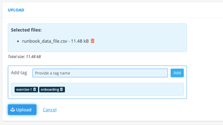
Navigate to File Management (Smart Integration) and Upload button on the top right, which leads you to a fairly intuitive upload UI.
When you’ve selected the file (for future reference: you can upload multiple files at once!), you get the option to add tags to the file(s). This allows you to easily search for files, for example files with the tag “exercise”. Hit the upload button and you can return to File Management to see that the file has been added.
ii)Datasource Classifier
Navigate to the Datasource Classifiers page (also Smart Integration).
With Datasource Classifiers, we can define a type of Datasource. We’re going to create one, but be aware: creating a Datasource Classifier is definite. I.e., you cannot delete / edit it once created. Before creating a datasource, you should always consider if the data you’re trying to get in the platform can get classified under an existing Datasource Classifier.
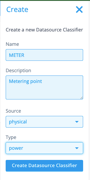
Below is the configuration we are going to use. The name of the Datasource Classifiers is what will appear on the Datasource when created. The data you are going to ingest now, is data from a meter. An appropriate name would hence be, “METER” (or “METERING_POINT”, “POWER”) etc.
The next important field is Source. You can choose between physical and virtual. We choose to set it to physical, since a meter can be considered the lowest point of aggregation, a physical device even. A virtual device would for example be the datasource with aggregated data for a network area.
The type is power, since we’re only ingesting power data. If we also had meters measuring gas consumption, we might have considered the option general.
iii)Channel Classifier
Navigate to Channel Classifier (surprise, also Smart Integration). A channel is where we store the timeseries data. With channel classifiers the system can express a type of timeseries, varying between the data(source) type and units.
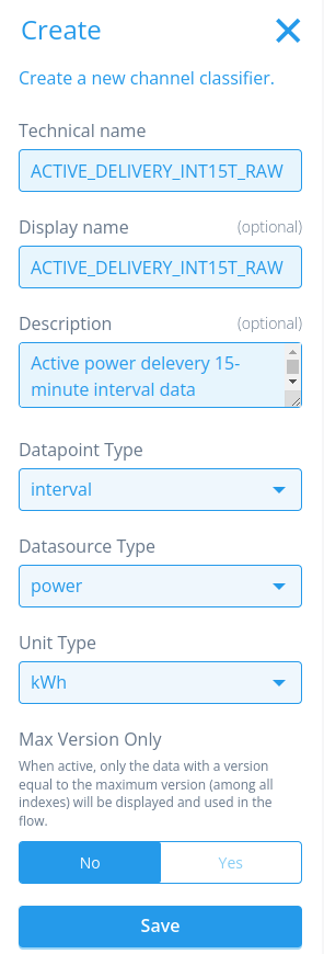
In this exercise we need a timeseries expressing consumption for a power meter. Our data are interval values: expressing delivered power for the last 15 minutes, not cumulative. The Datasource type is power, and the unit type is in kWh (the configured here is ACTIVE_DELIVERY_INT15T_RAW. The meaning of this channel name is that we are talking about active (not reactive power), delivery (so not redelivery, which means production) INT (interval data, not register data), 15T (one value per 15 minutes) RAW (unmodified, like the data that has been ingested).
iv)Rule Configuration
Navigate to Rules & Algorithms which you can find in Flow Management. We are going to need a rule later in the exercise to transform the timestamp (which has a local timezone) so that the system understands it is a local timezone, and what format to apply to transform it.
We already have an out-of-the-box transformation rule which will take care of the logic, we just need to configure the rule in the console. So click Create, and you should be directed to a configuration page.
Only configure the elements that are described in the exercise. If you have questions about other components, you can check for helpful articles in this Documentation site or ask the team.
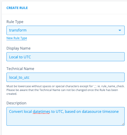
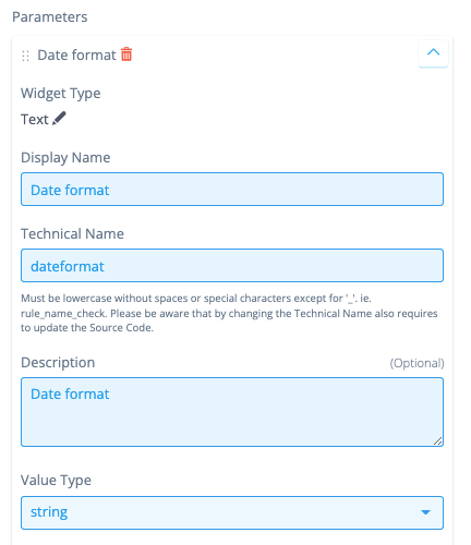
First, we configure the identifiable part: This will be a transformation rule, which is a type specifically used in Transformation Configurations. This type might not yet exist, but you can add it easily by clicking on "New Rule Type”. The name can be anything, but it’s good to stay close to its context, and relate it to the technical name.
If the rule is only configured in the frontend, the name can be anything (but it has to be snake_case), in this case you would have to store the python code in the code blob on the right.
The description is in this case mandatory: describe the rule’s purpose / behaviour.
Rule parameters can be configurable by adding them in the configuration. These rule parameters correspond directly with the parameters in the rule. That is why, again, the technical name is not flexible, but the name is. The date format will be the parameter of this rule, which is a string.
Hit save!
Then, add the codeblob below to the rule, and again save the rule configuration.
    """
    Copyright 2017-2023 Energyworx International B.V.
    """

    from energyworx_public.rule import AbstractTransformRule

    class LocalToUtc(AbstractTransformRule):
        def apply(self, dateformat, **kwargs):
            import pandas as pd

            if isinstance(self.dataframe, pd.Series):
                return self.dataframe

            dataframe = pd.to_datetime(self.dataframe.squeeze(axis=1), format=dateformat)

            result = []
            for timezone, df in dataframe.groupby(self.result['timezone']):
                if df.dt.tz is None:
                    df = df.dt.tz_localize(timezone, ambiguous='infer')
                result.append(df.dt.tz_convert('UTC'))

            return pd.concat(result)
v) Transformation Configuration (TC)
Navigate back to File Management and click on Details for the file that you have just uploaded. A menu on the right should pop up, and you can select Transformation Config...
You should be redirected to a new page, where you can configure the TC. Let’s first discuss what we are seeing here:
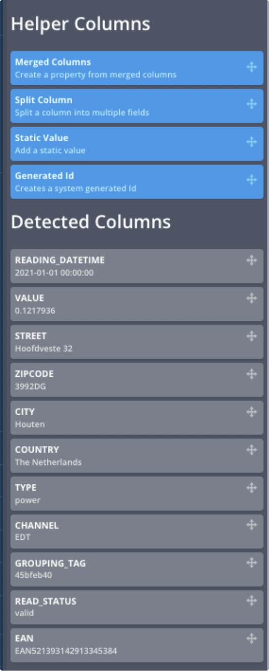
On the left We have the Helper Columns which allow you to add static values to the configuration, split columns, generate random id’s and to merge columns if you need the information in the same field. Below the Helper Columns we see the fields that the system could automatically detect in your file (this is now only possible for .csv files). This is a huge help when configuring the TC!
On the right you can create the configurations. There are all kinds of fields to fill out to have a valid configuration. Anything marked  has not been configured (correctly) yet. When it turns green, you’re good to go!
In the next step we’ll start with the configuration whilst explaining the fields.
vi) Configuring the TC
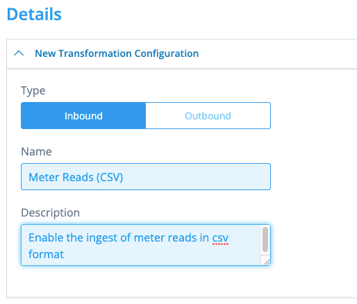
(a) Details
The first part of the configuration is for documentation’s sake: you should properly name the configuration, and document an apt description of the purpose of this TC. It can be anything, but let’s set a good example:
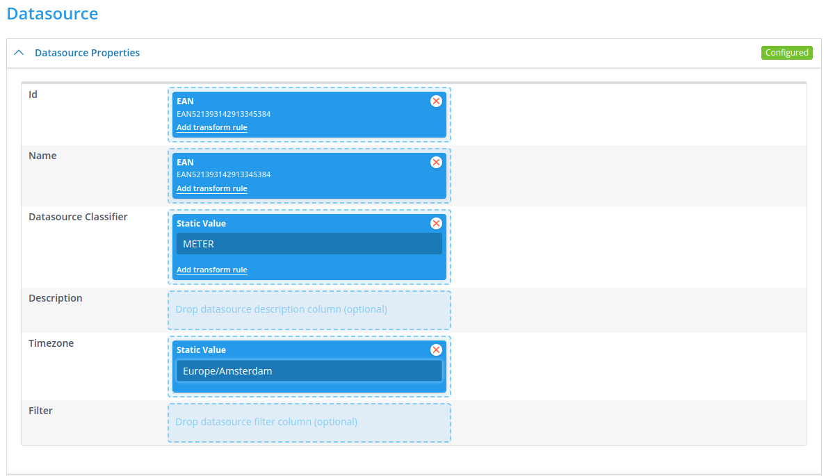
(b) Datasource
The datasource properties are a bit stricter: you have to use fields, and they are elementary in the terms of the creation of the datasource. The id is what we can identify a datasource with. E.g., if you need to pull data from a different datasource in a rule, you have to use the id to retrieve it. It follows that the id must be unique in the namespace.
We’re going to use some of the fields of our file. But you can also use static values, which we will use to set the timezone of the datasource. For a Datasource Classifier, you are going to use the one you’ve just configured: METER. This should be done with a static value. Meters have a physical location as well, which is why a datasource should also have a timezone configured. In this case we have to add it as a static value, but it might be possible that it can be derived from the file. The Timezone field allows you to view anything on the datasource in this timezone (and by default also in UTC)
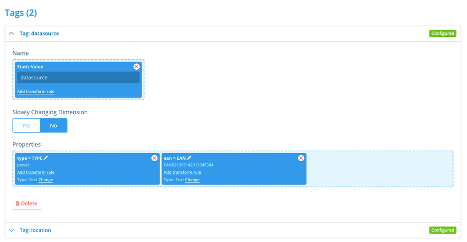
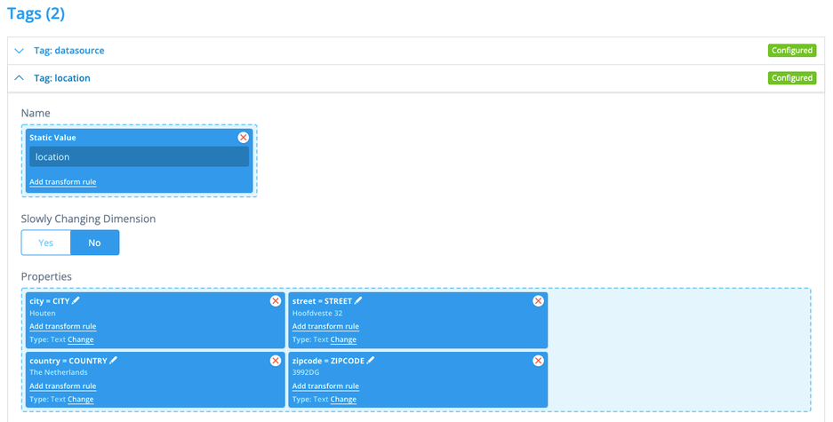
(c) Tags
With tags we can add metadata to the datasource. This kind of data either cannot be expressed by a timeseries, or it rarely changes. There is all kinds of information in our file, so we configure 2 tags:
datasource with some more datasource details, and location with location information. The name of the tag is a static value in this case, just drag and drop the other values in properties. You can leave the key of a property in upper case, but we tend to modify it to lower case (also useful if you want the key to be something completely different) by clicking on the pencil to edit.
(d) Channel
Now, the last part for this configuration is to get the timeseries data on the channel. Select the channel classifier (Find a Channel Classifier) that you have configured: ACTIVE_DELIVERY_INT15T_RAW. Drag the READING_DATETIME field to Timestamps and add the transform rule Local to UTC. To configure the parameters of this transform rule, click the cogwheel, and set the datetime format to the format in the file: %Y-%m-%d %H:%M:%S. Finally, add the VALUE field to Values.

Do not forget to save the Transformation Configuration!
vii) Configure the Market Adapter (MA)
Navigate to Market Adapters (Smart Integration), and hit Create.
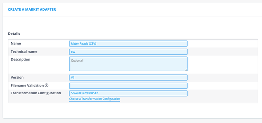
Configure the MA as shown below. But let us also briefly discuss each field that we filled out.
The name can be anything, but I like to make it relatable to the Transformation Configuration the Market Adapter is going to use.
Technical name is strict: this field directly corresponds to a folder & file in the platform. So it must exist. Lucky for us, there exists a csv.py file in the backend which holds a method to adapt csv data.
Version is also strict: this field directly corresponds to the class in the file. In this example/exercise, there exists a class V1 in the file csv.py.
Transformation Configuration: you need to select the Transformation Configuration that you have just configured, note that the id shown in the screenshot is most probably different than you have: these id’s are randomly generated. The ingest process will use this Transformation Configuration after adapting the data with the Market Adapter.
Properties allow us to fill parameters that the Market Adapter has in the backend.
For example, we can set the delimiter using the separator property, or to split the file in files with each split_lines lines to make use of the parallel processing capabilities of the platform. For this exercise, we tell the Market Adapter to split the file every 96 lines.
...and don’t forget to hit save!

viii) Ingest the file
Now everything should be set up for you to ingest your first file!
Navigate back to File Management and find your file. Click Ingest and the right side panel should appear. Here you can select what MA to use, you know which one to select.
Hit Ingest again, and you should get a message whether the trigger of the ingest was successful!
ix) Monitor
The easiest way to monitor your ingestion in the console is to check the Audit events. You navigate to Audit Events (just above Support in the menu on the left), where you can check whether any of the events are relevant to your ingest.
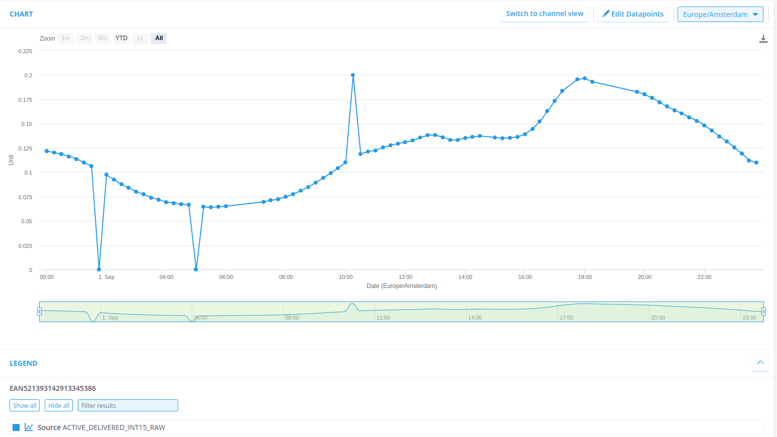
You can also check in Search Datasources to see if you can already locate your datasource (this can be found in Search at the top of the menu). Either directly hit the Search button in Search Datasources or enter the name of our datasource (EAN521393142913345387). You can then click on details and you should be directed to the datasource view.
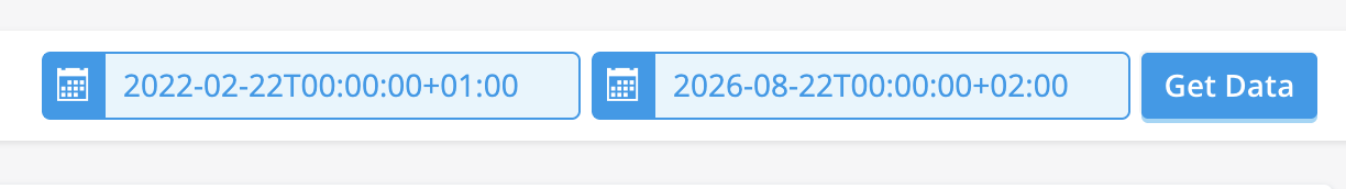
The data that we’ve ingested is from September 2023, so be sure to set your time range correctly and check if the data is indeed stored at Chart!
3. Running a Flow
For this exercise you’re going to configure a flow. Quick recap: flows are used to transform data into something valuable (now or for another process) by linking rules (written in Python) in sequences. You are going to apply the zero_reads rule to the datasource system has created in exercise (1).
i) Configure the standard_gap_check_validation rule
The standard_gap_check_validation rule is a base validation rule. It validates the data by checking for missing reads. These missing reads need to be flagged to eventually be estimated in the VEE process.
Navigate to Rules & Algorithms and create a new rule, this time, a validation rule. Name the rule appropriately and fill the code blob below.
    """
    Copyright 2017-2023 Energyworx International B.V.
    """
    import pandas as pd

    from energyworx.domain import DictWrapper, RuleResult
    from energyworx.rules.base_rule import AbstractRule


    class StandardGapCheckValidation(AbstractRule):
        def apply(self, data_frequency=pd.Timedelta("15min"), **kwargs):
            """ Checks for gaps for interval data. It uses the data_frequency
            argument as input. When values are missing, it creates a daterange
            and extends the existing dataframe index. It returns a series of
            flags, one flag for each (missing and present) datapoint.

            Args:
                data_frequency (pd.Timedelta): Specifies the time interval
                    that should be between readings.
                    defaults to 15 minutes.

            Returns:
                RuleResult(result=pd.Series); if gaps present; the
                    returning series will be longer than the original
            """
            import pandas as pd

            source_df = self.dataframe
            indices_to_check = pd.date_range(start=source_df.index.min(), end=source_df.index.max(), freq=data_frequency)
            missing_indices = indices_to_check[~indices_to_check.isin(source_df.index)]
            source_df.reindex(columns=list(source_df.columns.values) + ['FLAG'])
            flag_df = pd.DataFrame(index=indices_to_check)
            flag_df.loc[:, 'FLAG'] = DictWrapper()
            flag_df.loc[missing_indices, 'FLAG'] = DictWrapper(gap='True')
            flag_series = flag_df.loc[missing_indices, 'FLAG']

            return RuleResult(result=flag_series)
Note, the technical name should be snake case of the class name of this rule: StandardGapCheckRule → standard_gap_check_rule. Also, configure the parameter data frequency with a Text field. Don’t forget to configure the default value, which we here set to “15min”

Hit save. 😊
Fun fact: depending on the configurations of the environment, rules are cached for a certain amount of time. This means, if you hit save, the new version of an existing rule won’t become available for flows until that time has passed. This can be set in the Namespace Properties. For staging/demo environments it’s quite common to set this threshold pretty low, but production environments need to have this threshold higher to revert to a stable version before the new version takes effect.
ii) Configure the flow
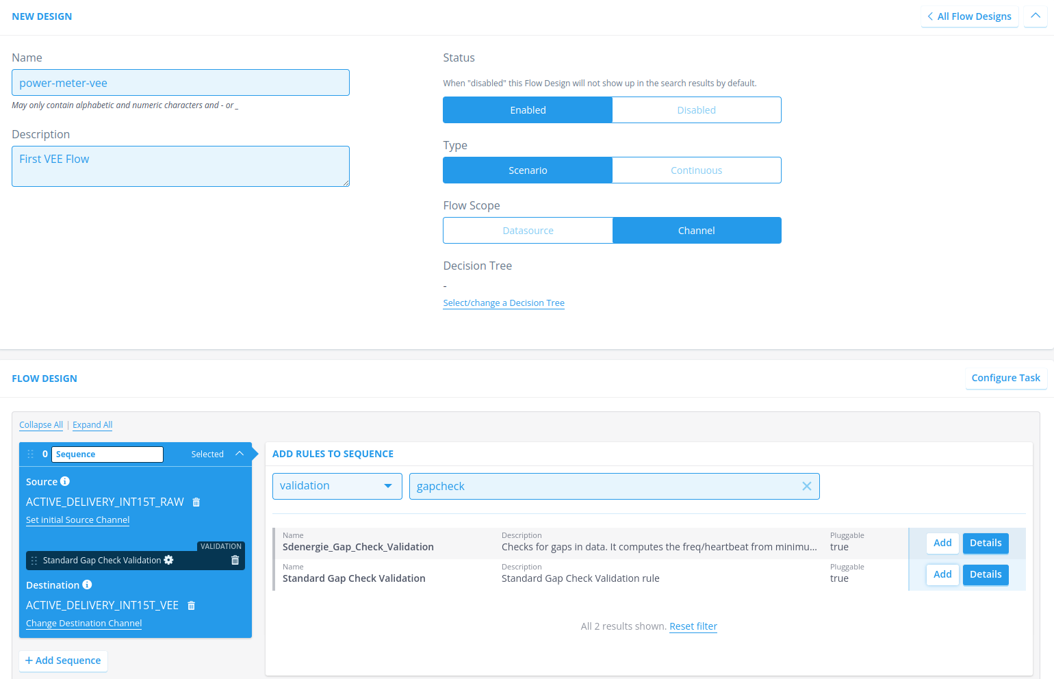
Navigate to Flow Designs and hit + New Design to start configuring a new flow configuration.
Name the flow appropriately, and adhere to the specified conditions, for example power-meter-vee
Add an apt description; within Energyworx we often use the term VEE for flows that perform checks on the data (Validation, Estimation, Edits).
Next, look at the sequence, and set the correct source channel. By setting the source channel you’re telling the system to make this channel available during the rule execution, but it also sets the class property self.source_column which is available during the rule execution (e.g., see line 35 in the code blob, self.source_column is used to retrieve a specific timeseries from the dataframe).
Add the gap check rule to the sequence
Add the store timeseries rule (under type storage) to the sequence: you have not configured this rule yourself, but this should already be available in your namespace. Additionally, set the Classifier parameter of this rule to the channel on which the annotations are going to be stored, which is the same channel as we are performing the flow on: ACTIVE_DELIVERY_INT15T_RAW.
Add a destination channel, which is also the channel we’re performing this check on.
Hit save
iii) Trigger the flow
There are 3 ways to start a flow manually:
In Search Datasources you can select the datasources you wish to trigger a flow on. Once selected, the option to trigger a flow appears at the top of the list: Start flow(s) for selection.
You can also navigate to the datasource and look for the Start Flow button. A side panel appears, and you can select a flow. Start the flow (and yes, you are sure you want to start it)
In the view of the flow design you can, at the top, also click Start Flow. This will lead you to a search page where you can select the datasources on which you want to trigger the flow.
Do not forget to apply the correct date range.
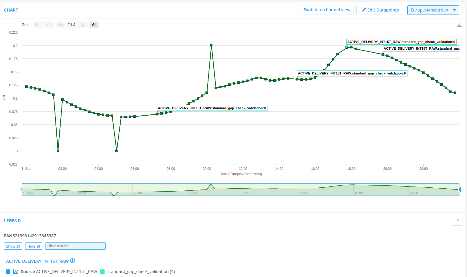
You can check the audit events on the datasource itself to track the progress of the flow. Once finished (all audit events are in), refresh the page to view the results of the flow in the graph, you should have 3 annotations:
4. Develop your own rule
This exercise will give you a push in the direction of rule creation, and test it out in a flow. As you might already have noticed: the data that you have ingested has more flaws than just gaps. Namely, there are also values being zero, and there is an outlier! Now, we can exercise creating rules to flag these defects.
Before going to code, we want to explain a little bit about annotations. Annotations are a concept which ‘annotate’ or ‘flag’ a datapoint in a timeseries. This is done as the result of a rule, specifically, it is a returned as a series of dictionaries or assigned during data ingestion.
The following apply function within a rule would generate an annotation for each index in the dataframe:
from energyworx.rules.base_rule import AbstractRule

from energyworx.domain import RuleResult


    class SampleRule(AbstractRule):

      def apply(self, **kwargs):

        # Sets the dastaframe provided to the rule as df.
        df = self.dataframe

        # Creates a column in the dataframe and, for every index, creates a dictionary
        df['sample_annotation'] = {
          'type': 'annotation sample',
          'detail': 'annotation detail'
        }

      # Returns a pd.Series, which is the column with the annotation generated.
      return RuleResult(result=df['sample_annotation'])
This has as result annotations like this:
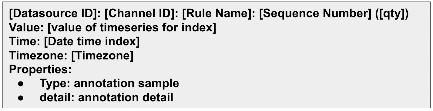
What’s also good to know, is that you can print debugging messages from the rule to the audit events using self.rule_logger.debug(“message”).
For this exercise, I would advise to just create a branch locally and not push it to the remote, as it is just an exercise, and the code will not have to be merged to develop. I.e. checkout the develop branch, make sure you’re up to date and create a new branch locally.
Depending on the rule you’re going to create, the rule’s class has to inherit from any of the configured rule classes.
As to the actual development of the rule, there are two ways to go about it:
Debugging and developing on the platform. Of course, this will only work for very small examples and should now only be done for learning how to work with the platform. At a later stage, local debugging works more efficiently.
Start with a unit test and start building your logic from there. This does not take away the need to test your rule in a flow!
    import pandas as pd
    from energyworx.rules.validation.some_awesome_rule import SomeAwesomeRule # <-- import the rule you're unit-testing
    from parameterized import parameterized # <-- this allows for testing multiple scenarios in the same test setting
    from tests.unit.rules.test_rules import RulesTest # <-- a class from which the test will inherit, it mocks/creates some objects in the framework to save you the time!

    class TestSomeAwesomeRule(RulesTest):

      rule_name = 'some_awesome_rule'

      @parameterized.expand([
        ('test_case_1', data_in1, expected1),
        ('test_case_2', data_in2, expected2)
      ])

      def test_default(self, name, data_in, expected):
        rule = SomeAwesomeRule(datasource=self.datasource, dataframe=data, source_column='TEST')
        result = rule.apply() # <- every rule has an apply function where the logic is applied

        # perform the test checks
        # many more assertions are available because RulesTest inherits from unittest.TestCase https://docs.python.org/3/library/unittest.html#unittest.TestCase
        self.assertEqual(result.result, expected)
Unit testing can become quite complex, this is just a simple example.
4.1 Exercise: write 2 validation rules
Rules that perform a check on the data are generally classified as validation rules. In this exercise you are going to develop 2 validation rules.
| Rule | Description | User Story (development guidelines) |
|---|---|---|
| Zero_reads_exercise | Find all values that are (close to) zero, and store these as annotations. | As a functional user I want to be able to detect zero reads in time series data so that we can have some measure of the quality of the data, and that they can be estimated. As output, it must show me an annotation on each datapoint being a zero read on the source time series. A zero read is defined as a value that is very close to zero. Only float rounding errors should be able to explain values just a little bit bigger than zero. For each zero read timestamp, there should be an annotation returned in the rule. The framework should take care of creating a proper annotations. |
| outlier_check_exercise | Based on the data available, detect the outlier. A simple method is good enough, but creativity is alway appreciated! | As a functional user I want to easily see for a timeseries if any point might be considered an outlier. I would like a(nother) validation rule that checks the data for potential outliers. The method may be something simple for the purpose of this exercise, then adhere to the following requirements: for each outlier, write an annotation on the timestamp report the metrics of the decision on the annotation, e.g., a calculated score and/or threshold If you feel like putting in a little bit more time (and a little bit more statistically and/or mathematically inclined) you can develop also something more sophisticated. For that purpose, here are some additional requirements: The method should be robust against changing patterns (e.g., consistent higher usage on Fridays should not be flagged as an outlier) |
Add these rules to the previously configured VEE flow, and try it out!